Perform a biosensor model fit on response vs. concentration data of a single sample.
Source:R/dose-response-analysis.R
fl.drFitModel.Rdfl.drFitModel fits the biosensor model proposed by Meyer et al. (2019) to the provided response (e.g., max_slope.spline vs. concentration data to determine the leakiness, sensitivity, induction fold-change, and cooperativity.
Usage
fl.drFitModel(conc, test, drID = "undefined", control = fl.control())Arguments
- conc
Vector of concentration values.
- test
Vector of response parameter values of the same length as
conc.- drID
(Character) The name of the analyzed condition
- control
A
fl.controlobject created withfl.control, defining relevant fitting options.
Value
A drFitFLModel object.
- raw.conc
Raw data provided to the function as
conc.- raw.test
Raw data for the response parameter provided to the function as
test.- drID
(Character) Identifies the tested condition
- fit.conc
Fitted concentration values.
- fit.test
Fitted response values.
- model
nlsobject generated by thenlsLMfunction.- parameters
List of parameters estimated from dose response curve fit.
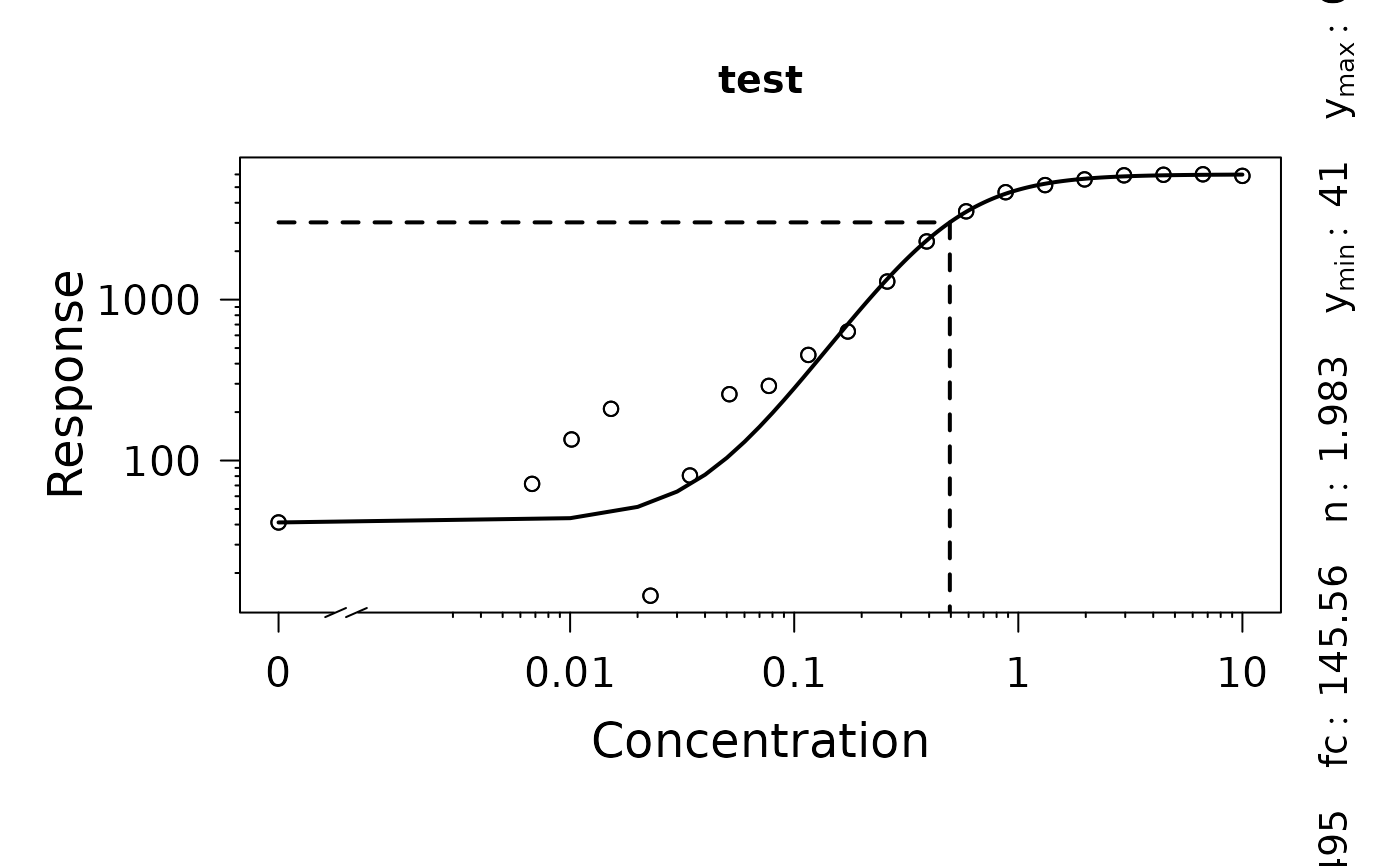
yEC50: Response value related to EC50.y.min: Minimum fluorescence ('leakiness', if lowest concentration is 0).y.max: Maximum fluorescence.fc: Fold change (y.maxdivided byy.min).K: Concentration at half-maximal response ('sensitivity').n: Cooperativity.yEC50.orig: Response value for EC50 in original scale, if a transformation was applied.K.orig: K in original scale, if a transformation was applied.test.nm: Test identifier extracted fromtest.
- fitFlag
(Logical) Indicates whether a spline could fitted successfully to data.
- reliable
(Logical) Indicates whether the performed fit is reliable (to be set manually).
- control
Object of class
fl.controlcreated with the call offl.control.
Use plot.drFitModel to visualize the model fit.
References
Meyer, A.J., Segall-Shapiro, T.H., Glassey, E. et al. Escherichia coli “Marionette” strains with 12 highly optimized small-molecule sensors. Nat Chem Biol 15, 196–204 (2019). DOI: 10.1038/s41589-018-0168-3
Examples
# Create concentration values via a serial dilution
conc <- c(0, rev(unlist(lapply(1:18, function(x) 10*(2/3)^x))),10)

# Simulate response values via biosensor equation
response <- biosensor.eq(conc, y.min = 110, y.max = 6000, K = 0.5, n = 2) +
            0.01*6000*rnorm(10)

# Perform fit
TestRun <- fl.drFitModel(conc, response, drID = 'test', control = fl.control())
#>
#>
#> === Dose response curve estimation ================
#> --- EC 50 -----------------------------------------
#> --> test
#> sensitivity: 0.495 | yEC50: 3021 | fold change: 145.56 | leakiness: 41.2
#>
#>

print(summary(TestRun))
#>      yEC50    y.min    y.max       fc         K        n yEC50.orig    K.orig
#> 1 3020.854 41.22442 6000.484 145.5566 0.4948616 1.982843   3020.854 0.4948616
#>   test
#> 1   NA
plot(TestRun)
