Perform a smooth spline fit on response vs. concentration data of a single sample
Source:R/dose-response-analysis.R
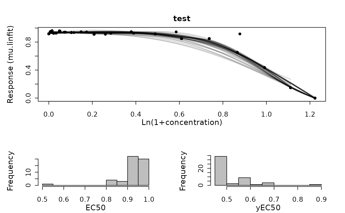
growth.drBootSpline.Rdgrowth.drBootSpline resamples the values in a dataset with replacement and performs a spline fit for each bootstrap sample to determine the EC50.
Usage
growth.drBootSpline(conc, test, drID = "undefined", control = growth.control())Arguments
- conc
Vector of concentration values.
- test
Vector of response parameter values of the same length as
conc.- drID
(Character) The name of the analyzed sample.
- control
A
grofit.controlobject created withgrowth.control, defining relevant fitting options.
Value
An object of class drBootSpline containing a distribution of growth parameters and
a drFitSpline object for each bootstrap sample. Use plot.drBootSpline
to visualize all bootstrapping splines as well as the distribution of EC50.
- raw.conc
Raw data provided to the function as
conc.- raw.test
Raw data for the response parameter provided to the function as
test.- drID
(Character) Identifies the tested condition.
- boot.conc
Table of concentration values per column, resulting from each spline fit of the bootstrap.
- boot.test
Table of response values per column, resulting from each spline fit of the bootstrap.
- boot.drSpline
List containing all
drFitSplineobjects generated by the call ofgrowth.drFitSpline.- ec50.boot
Vector of estimated EC50 values from each bootstrap entry.
- ec50y.boot
Vector of estimated response at EC50 values from each bootstrap entry.
- BootFlag
(Logical) Indicates the success of the bootstrapping operation.
- control
Object of class
grofit.controlcontaining list of options passed to the function ascontrol.
References
Matthias Kahm, Guido Hasenbrink, Hella Lichtenberg-Frate, Jost Ludwig, Maik Kschischo (2010). grofit: Fitting Biological Growth Curves with R. Journal of Statistical Software, 33(7), 1-21. DOI: 10.18637/jss.v033.i07
See also
Other dose-response analysis functions:
flFit(),
growth.drFitSpline(),
growth.gcFit(),
growth.workflow()
Examples
conc <- c(0, rev(unlist(lapply(1:18, function(x) 10*(2/3)^x))),10)
response <- c(1/(1+exp(-0.7*(4-conc[-20])))+rnorm(19)/50, 0)

TestRun <- growth.drBootSpline(conc, response, drID = 'test',
               control = growth.control(log.x.dr = TRUE, smooth.dr = 0.8,
                                        nboot.dr = 50))
#> === Bootstrapping of dose response curve ==========
#> --- EC 50 -----------------------------------------
#>
#> Mean  :  0.921992506861759 StDev :  0.0704571905257327
#> 90% CI:  0.919674465293462 90% CI:  0.924310548430055
#> 95% CI:  0.91923058499315 95% CI:  0.924754428730367
#>
#>
#> --- EC 50 in original scale -----------------------
#>
#> Mean  :  1.5142951526126
#> 90% CI:  1.50847366176949 90% CI:  1.52013015356593
#> 95% CI:  1.50736044681255 95% CI:  1.52124903800233
#>

print(summary(TestRun))
#>   drboot.meanEC50 drboot.sdEC50 drboot.meanEC50y drboot.sdEC50y
#> 1       0.9219925    0.07045719        0.5145351     0.08320139
#>   drboot.ci90EC50.lo drboot.ci90EC50.up drboot.ci95EC50.lo drboot.ci95EC50.up
#> 1          0.8060904           1.037895          0.7838964           1.060089
#>   drboot.meanEC50.orig drboot.ci90EC50.orig.lo drboot.ci90EC50.orig.up
#> 1             1.514295                1.239137                1.823267
#>   drboot.ci95EC50.orig.lo drboot.ci95EC50.orig.up
#> 1                1.189989                1.886627
plot(TestRun, combine = TRUE)