Data fit via a heuristic linear method

Determine maximum slopes from using a heuristic approach similar to the ``growth rates made easy''-method of Hall et al. (2013).

Usage

flFitLinear(
  time = NULL,
  growth = NULL,
  fl_data,
  ID = "undefined",
  quota = 0.95,
  control = fl.control(x_type = c("growth", "time"), log.x.lin = FALSE, log.y.lin =
    FALSE, t0 = 0, min.growth = NA, lin.h = NULL, lin.R2 = 0.98, lin.RSD = 0.05, lin.dY =
    0.05, biphasic = FALSE)
)

Arguments

time: Vector of the independent time variable (if x_type = "time" in control object).
growth: Vector of the independent time growth (if x_type = "growth" in control object).
fl_data: Vector of the dependent fluorescence variable.
ID: (Character) The name of the analyzed sample.
quota: (Numeric, between 0 an 1) Define what fraction of max_slope the slope of regression windows adjacent to the window with highest slope should have to be included in the overall linear fit.
control: A fl.control object created with fl.control, defining relevant fitting options.

Value

A gcFitLinear object with parameters of the fit. The lag time is estimated as the intersection between the fit and the horizontal line with \(y=y_0\), where y0 is the first value of the dependent variable. Use plot.gcFitSpline to visualize the linear fit.

raw.x: Filtered x values used for the spline fit.
raw.fl: Filtered fluorescence values used for the spline fit.
filt.x: Filtered x values.
filt.fl: Filtered fluorescence values.
ID: (Character) Identifies the tested sample.
FUN: Linear function used for plotting the tangent at mumax.
fit: lm object; result of the final call of lm to perform the linear regression.
par: List of determined fluorescence parameters.

y0: Minimum fluorescence value considered for the heuristic linear method.
dY: Difference in maximum fluorescence and minimum fluorescence
A: Maximum fluorescence
y0_lm: Intersection of the linear fit with the abscissa.
max_slope: Maximum slope of the linear fit.
tD: Doubling time.
slope.se: Standard error of the maximum slope.
lag: Lag X.
x.max_start: X value of the first data point within the window used for the linear regression.
x.max_end: X value of the last data point within the window used for the linear regression.
x.turn: For biphasic: X at the inflection point that separates two phases.
max.slope2: For biphasic: Slope of the second phase.
tD2: Doubling time of the second phase.
y0_lm2: For biphasic: Intersection of the linear fit of the second phase with the abscissa.
lag2: For biphasic: Lag time determined for the second phase..
x.max2_start: For biphasic: X value of the first data point within the window used for the linear regression of the second phase.
x.max2_end: For biphasic: X value of the last data point within the window used for the linear regression of the second phase.

ndx: Index of data points used for the linear regression.
ndx2: Index of data points used for the linear regression for the second phase.
control: Object of class grofit.control containing list of options passed to the function as control.
rsquared: R² of the linear regression.
rsquared2: R² of the linear regression for the second phase.
fitFlag: (Logical) Indicates whether linear regression was successfully performed on the data.
fitFlag2: (Logical) Indicates whether a second phase was identified.
reliable: (Logical) Indicates whether the performed fit is reliable (to be set manually).

References

Hall, BG., Acar, H, Nandipati, A and Barlow, M (2014) Growth Rates Made Easy. Mol. Biol. Evol. 31: 232-38, DOI: 10.1093/molbev/mst187

Petzoldt T (2022). growthrates: Estimate Growth Rates from Experimental Data. R package version 0.8.3, https://CRAN.R-project.org/package=growthrates.

Examples

# load example dataset
input <- read_data(data.growth = system.file("lac_promoters.xlsx", package = "QurvE"),
                   data.fl = system.file("lac_promoters.xlsx", package = "QurvE"),
                   sheet.growth = 1,
                   sheet.fl = 2 )
#> Sample data are stored in columns. If they are stored in row format, please run read_data() with data.format = 'row'.

# Extract time and normalized fluorescence data for single sample
time <- input$time[4,]
data <- input$norm.fluorescence[4,-(1:3)] # Remove identifier columns

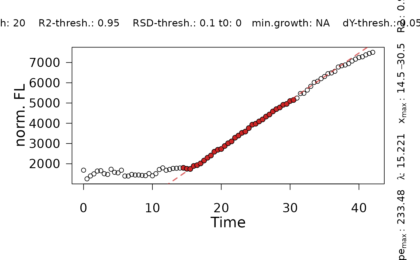
# Perform linear fit
TestFit <- flFitLinear(time = time,
                       fl_data = data,
                       ID = "TestFit",
                       control = fl.control(fit.opt = "l", x_type = "time",
                       lin.R2 = 0.95, lin.RSD = 0.1,
                       lin.h = 20))

plot(TestFit)