Combine different groups of samples into a single plot
Source:R/fluorescence_plots.R
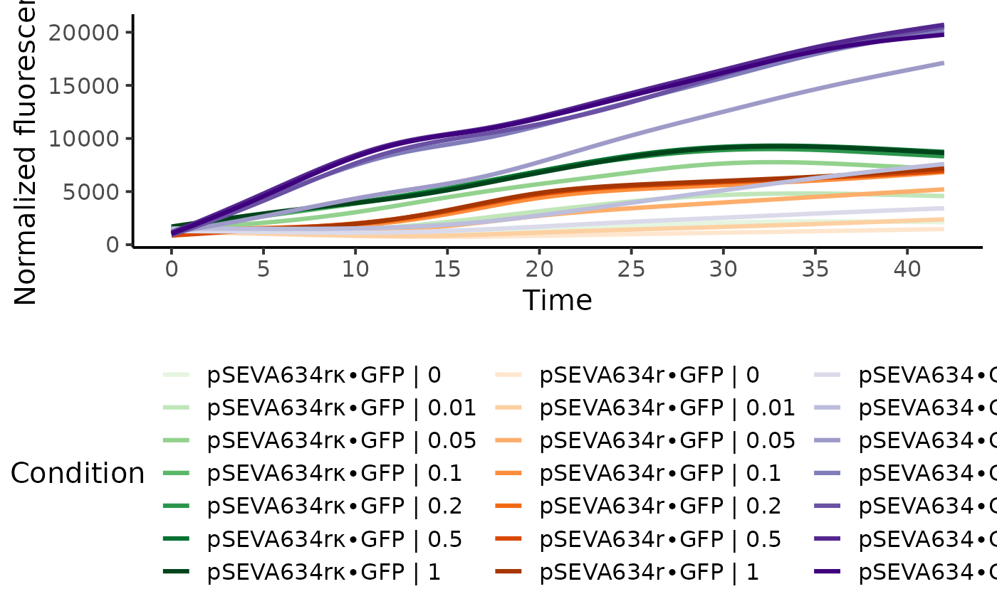
plot.flFitRes.RdVisualize fluorescence, normalized fluorescence, or spline fits of multiple sample groups in a single plot.
Usage
# S3 method for flFitRes
plot(
  x,
  data.type = c("spline", "raw", "norm.fl"),
  IDs = NULL,
  names = NULL,
  conc = NULL,
  mean = TRUE,
  exclude.nm = NULL,
  exclude.conc = NULL,
  log.y = FALSE,
  deriv = FALSE,
  n.ybreaks = 6,
  colors = NULL,
  color_groups = TRUE,
  group_pals = c("Green", "Orange", "Purple", "Magenta", "Grey", "Blue", "Grey", "Red",
    "Cyan", "Brown", "Mint"),
  basesize = 20,
  y.lim = NULL,
  x.lim = NULL,
  y.title = NULL,
  x.title = NULL,
  y.lim.deriv = NULL,
  y.title.deriv = NULL,
  lwd = 1.1,
  legend.position = "bottom",
  legend.ncol = 2,
  plot = TRUE,
  export = FALSE,
  height = NULL,
  width = NULL,
  out.dir = NULL,
  out.nm = NULL,
  ...
)

# S3 method for flFit
plot(
  x,
  data.type = c("spline", "raw", "norm.fl"),
  IDs = NULL,
  names = NULL,
  conc = NULL,
  mean = TRUE,
  exclude.nm = NULL,
  exclude.conc = NULL,
  log.y = FALSE,
  deriv = FALSE,
  n.ybreaks = 6,
  colors = NULL,
  color_groups = TRUE,
  group_pals = c("Green", "Orange", "Purple", "Magenta", "Grey", "Blue", "Grey", "Red",
    "Cyan", "Brown", "Mint"),
  basesize = 20,
  y.lim = NULL,
  x.lim = NULL,
  y.title = NULL,
  x.title = NULL,
  y.lim.deriv = NULL,
  y.title.deriv = NULL,
  lwd = 1.1,
  legend.position = "bottom",
  legend.ncol = 2,
  plot = TRUE,
  export = FALSE,
  height = NULL,
  width = NULL,
  out.dir = NULL,
  out.nm = NULL,
  ...
)
Arguments
- x
A
flFitRes,flFit, orgrodataobject created withfl.workflowcontaining fluorescence data.- data.type
(Character) Indicate, which type of fluorescence data should be displayed.
- IDs
(String or vector of strings) Define samples or groups (if
mean = TRUE) to combine into a single plot based on exact matches with entries in thelabelorconditioncolumns ofgrofit$expdesign.- names
(String or vector of strings) Define groups to combine into a single plot. Partial matches with sample/group names are accepted. If
NULL, all samples are considered. Note: Ensure to use unique substrings to extract groups of interest. If the name of one condition is included in its entirety within the name of other conditions, it cannot be extracted individually.- conc
(Numeric or numeric vector) Define concentrations to combine into a single plot. If
NULL, all concentrations are considered. Note: Ensure to use unique concentration values to extract groups of interest. If the concentration value of one condition is included in its entirety within the name of other conditions (e.g., the dataset contains '1', '10', and '100',code = 10will select both '10 and '100'), it cannot be extracted individually.- mean
(Logical) Display the mean and standard deviation of groups with replicates (
TRUE) or plot each sample individually (FALSE)?- exclude.nm
(String or vector of strings) Define groups to exclude from the plot. Partial matches with sample/group names are accepted.
- exclude.conc
(Numeric or numeric vector) Define concentrations to exclude from the plot.
- log.y
(Logical) Log-transform the y-axis of the plot (
TRUE) or not (FALSE)?- deriv
(Logical) Show derivatives over time in a separate panel below the plot (
TRUE) or not (FALSE)?- n.ybreaks
(Numeric) Number of breaks on the y-axis. The breaks are generated using
axisTicks(). Thus, the final number of breaks can deviate from the user input.- colors
(vector of strings) Define a color palette used to draw the plots. If
NULL, default palettes are chosen based on the number of groups/samples within the plot. Note: The number of provided colors should at least match the number of groups/samples.- color_groups
(Logical) Shall samples within the same group but with different concentrations be shown in different shades of the same color?
- group_pals
(String vector) Define the colors used to display sample groups with identical concentrations. The number of selected color palettes must be at least the number of displayed groups. The order of the chosen palettes corresponds to the oder of conditions in the legend. Available options: "Green", "Oranges", "Purple", "Cyan", "Grey", "Red", "Blue", and "Magenta".
- basesize
(Numeric) Base font size.
- y.lim
(Numeric vector with two elements) Optional: Provide the lower (
l) and upper (u) bounds of the y-axis of the fluorescence curve plot as a vector in the formc(l, u). If only the lower or upper bound should be fixed, providec(l, NA)orc(NA, u), respectively.- x.lim
(Numeric vector with two elements) Optional: Provide the lower (
l) and upper (u) bounds of the x-axis of both fluorescence curve and derivative plots as a vector in the formc(l, u). If only the lower or upper bound should be fixed, providec(l, NA)orc(NA, u), respectively.- y.title
(Character) Optional: Provide a title for the y-axis of the fluorescence curve plot.
- x.title
(Character) Optional: Provide a title for the x-axis of both fluorescence curve and derivative plots.
- y.lim.deriv
(Numeric vector with two elements) Optional: Provide the lower (
l) and upper (u) bounds on the y-axis of the derivative plot as a vector in the formc(l, u). If only the lower or upper bound should be fixed, providec(l, NA)orc(NA, u), respectively.- y.title.deriv
(Character) Optional: Provide a title for the y-axis of the derivative plot.
- lwd
(Numeric) Line width of the individual plots.
- legend.position
(Character) Position of the legend. One of "bottom", "top", "left", "right".
- legend.ncol
(Numeric) Number of columns in the legend.
- plot
(Logical) Show the generated plot in the
Plotspane (TRUE) or not (FALSE). IfFALSE, a ggplot object is returned.- export
(Logical) Export the generated plot as PDF and PNG files (
TRUE) or not (FALSE).- height
(Numeric) Height of the exported image in inches.
- width
(Numeric) Width of the exported image in inches.
- out.dir
(Character) Name or path to a folder in which the exported files are stored. If
NULL, a "Plots" folder is created in the current working directory to store the files in.- out.nm
(Character) The name of the PDF and PNG files if
export = TRUE. IfNULL, a name will be automatically generated including the chosen parameter.- ...
Additional arguments. This has currently no effect and is only meant to fulfill the requirements of a generic function.
Value
A plot with all curves (nonparametric fits, raw fluorescence measurements, or raw normalized fluorescence over time) in a flFitRes object created with fl.workflow, with replicates combined by the group averages (if mean = TRUE) or not (mean = FALSE).
A plot with all curves (raw fluorescence measurements or raw normalized fluorescence over time) in a flFit object with flFit, with replicates combined by the group averages (if mean = TRUE) or not (mean = FALSE).
Examples
# \donttest{
# load example dataset
input <- read_data(data.growth = system.file("lac_promoters.xlsx", package = "QurvE"),
                   data.fl = system.file("lac_promoters.xlsx", package = "QurvE"),
                   sheet.growth = 1,
                   sheet.fl = 2 )
#> Sample data are stored in columns. If they are stored in row format, please run read_data() with data.format = 'row'.

# Run workflow
res <- fl.workflow(grodata = input, ec50 = FALSE, fit.opt = "s",
                   x_type = "time", norm_fl = TRUE,
                   dr.parameter = "max_slope.spline",
                   suppress.messages = TRUE,
                   parallelize = FALSE)

plot(res, legend.ncol = 3, basesize = 15)

# }

# load example dataset
input <- read_data(data.growth = system.file("lac_promoters.xlsx", package = "QurvE"),
                   data.fl = system.file("lac_promoters.xlsx", package = "QurvE"),
                   sheet.growth = 1,
                   sheet.fl = 2 )
#> Sample data are stored in columns. If they are stored in row format, please run read_data() with data.format = 'row'.

# Run curve fitting workflow
res <- flFit(fl_data = input$norm.fluorescence,
             time = input$time,
             parallelize = FALSE,
             control = fl.control(fit.opt = "s", suppress.messages = TRUE,
             x_type = "time", norm_fl = TRUE))

plot(res, legend.ncol = 3, basesize = 15)
# }
# load example dataset
input <- read_data(data.growth = system.file("lac_promoters.xlsx", package = "QurvE"),
data.fl = system.file("lac_promoters.xlsx", package = "QurvE"),
sheet.growth = 1,
sheet.fl = 2 )
#> Sample data are stored in columns. If they are stored in row format, please run read_data() with data.format = 'row'.
# Run curve fitting workflow
res <- flFit(fl_data = input$norm.fluorescence,
time = input$time,
parallelize = FALSE,
control = fl.control(fit.opt = "s", suppress.messages = TRUE,
x_type = "time", norm_fl = TRUE))
plot(res, legend.ncol = 3, basesize = 15)