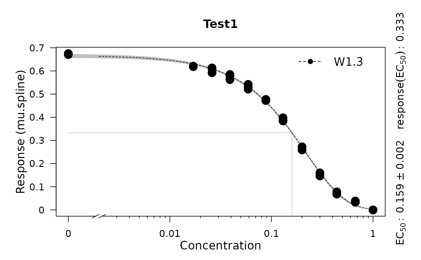
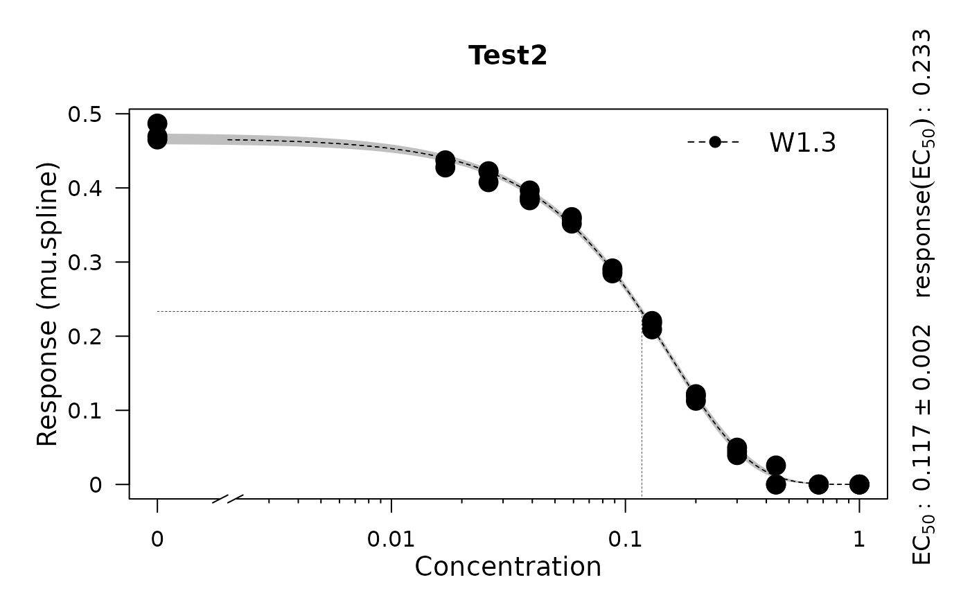
The function calls the baranyi function to generate curves between time zero and t and adds some random noise to the x- and y-axes. The three growth parameters given as input values will be slightly changed to produce different growth curves. The resulting datasets can be used to test the growth.workflow function.

The function calls the baranyi function to generate curves between time zero and t and adds some random noise to the x- and y-axes. The three growth parameters given as input values will be slightly changed to produce different growth curves. The resulting datasets can be used to test the growth.workflow function.

Usage

rdm.data(d, y0 = 0.05, tmax = 24, mu = 0.6, lambda = 5, A = 3, label = "Test1")

Arguments

d: Numeric value, number of data sets. If d is a vector, only the first entry is used.
y0: Numeric value, start growth. If t is a vector, only the first entry is used.
tmax: Numeric value, number of time points per data set. If t is a vector, only the first entry is used.
mu: Numeric value, maximum slope. If mu is a vector, only the first entry is used.
lambda: Numeric value, lag-phase. If lambda is a vector, only the first entry is used.
A: Numeric value, maximum growth. If A is a vector, only the first entry is used.
label: Character string, condition label If label is a vector, only the first entry is used.

Value

A list containing simulated data for three tests (e.g., 'organisms'):

time: numeric matrix of size dxt, each row represent the time points for which growth data is simulated and stored in each row of data.
data: data.frame of size dx(3+t), 1. column, character as an experiment identifier; 2. column: Replicate number; 3. column: concentration of substrate of a compound under which the experiment is obtained; 4.-(3+t). column: growth data corresponding to the time points in time.

References

Matthias Kahm, Guido Hasenbrink, Hella Lichtenberg-Frate, Jost Ludwig, Maik Kschischo (2010). grofit: Fitting Biological Growth Curves with R. Journal of Statistical Software, 33(7), 1-21. DOI: 10.18637/jss.v033.i07

Examples

# Create random growth data set
rnd.data1 <- rdm.data(d = 35, mu = 0.8, A = 5, label = 'Test1')
rnd.data2 <- rdm.data(d = 35, mu = 0.6, A = 4.5, label = 'Test2')

rnd.data <- list()
rnd.data[['time']] <- rbind(rnd.data1$time, rnd.data2$time)
rnd.data[['data']] <- rbind(rnd.data1$data, rnd.data2$data)

# Run growth curve analysis workflow
gcFit <- growth.gcFit(time = rnd.data$time,
                       data = rnd.data$data,
                       parallelize = FALSE,
                       control = growth.control(fit.opt = 's',
                                                suppress.messages = TRUE))

# \donttest{
# Perform dose-response analysis
drFit <- growth.drFit(gcTable = gcFit$gcTable,
             control = growth.control(dr.parameter = 'mu.spline'))
#> 
#> === EC 50 Estimation ==============================
#> ---------------------------------------------------
#> --> Checking data ...
#> --> Number of distinct tests found: 2 
#> --> Valid datasets per test: 
#>       TestID Number
#>       Test1  35    
#>       Test2  35    

# Inspect results
summary(drFit)
#>    Test log.x log.y Samples EC50.Estimate EC50.Std..Error EC50.Lower EC50.Upper
#> 1 Test1 FALSE FALSE       0     0.1590948     0.002450329  0.1541037  0.1640860
#> 2 Test2 FALSE FALSE       0     0.1174462     0.001950640  0.1134728  0.1214195
#>       yEC50      test model
#> 1 0.3330462 mu.spline  W1.3
#> 2 0.2334314 mu.spline  W1.3
plot(drFit)


# }