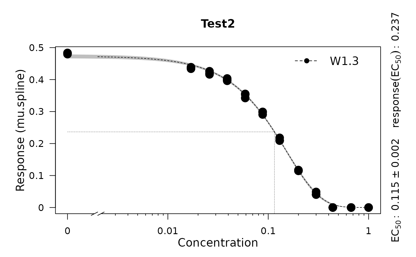
Perform a dose-response analysis on response vs. concentration data

growth.drFit serves to determine dose-response curves on every condition in a dataset. The response parameter can be chosen from every physiological parameter in a gcTable table which is obtained via growth.gcFit. growth.drFit calls the functions growth.drFitSpline and growth.drBootSpline, or growth.drFitModel to generate a table with estimates for EC50 and respecting statistics.

Usage

growth.drFit(
  gcTable,
  control = growth.control(dr.method = "model", dr.model = c("gammadr", "multi2", "LL.2",
    "LL.3", "LL.4", "LL.5", "W1.2", "W1.3", "W1.4", "W2.2", "W2.3", "W2.4", "LL.3u",
    "LL2.2", "LL2.3", "LL2.3u", "LL2.4", "LL2.5", "AR.2", "AR.3", "MM.2"),
    dr.have.atleast = 6, dr.parameter = "mu.linear", nboot.dr = 0, smooth.dr = NULL,
    log.x.dr = FALSE, log.y.dr = FALSE)
)

Arguments

gcTable: A dataframe containing the data for the dose-response curve estimation. Such table of class gcTable can be obtained by running growth.gcFit.
control: A grofit.control object created with growth.control, defining relevant fitting options.
dr.method: (Character) Define the method used to perform a dose-responde analysis: smooth spline fit ('spline') or model fitting ('model').
dr.model: (Character) Provide a list of models from the R package 'drc' to include in the dose-response analysis (if dr.method = 'model'). If more than one model is provided, the best-fitting model will be chosen based on the Akaike Information Criterion.
dr.have.atleast: (Numeric) Minimum number of different values for the response parameter one should have for estimating a dose response curve. Note: All fit procedures require at least six unique values. Default: 6.
dr.parameter: (Character or numeric) The response parameter in the output table to be used for creating a dose response curve. See growth.drFit for further details. Default: 'mu.linfit', which represents the maximum slope of the linear regression. Typical options include: 'mu.linfit', 'lambda.linfit', 'dY.linfit', 'mu.spline', 'dY.spline', 'mu.model', and 'A.model'.
smooth.dr: (Numeric) Smoothing parameter used in the spline fit by smooth.spline during dose response curve estimation. Usually (not necessesary) in (0; 1]. See smooth.spline for further details. Default: NULL.
log.x.dr: (Logical) Indicates whether ln(x+1) should be applied to the concentration data of the dose response curves. Default: FALSE.
log.y.dr: (Logical) Indicates whether ln(y+1) should be applied to the response data of the dose response curves. Default: FALSE.
nboot.dr: (Numeric) Defines the number of bootstrap samples for EC50 estimation. Use nboot.dr = 0 to disable bootstrapping. Default: 0.

Value

An object of class drFit.

raw.data: Data that passed to the function as gcTable.
drTable: Dataframe containing condition identifiers, fit options, and results of the dose-response analysis.
drBootSplines: List of all drBootSpline objects generated by the call of growth.drBootSpline for each distinct experiment.
drFittedSplines: List of all drFitSpline objects generated by the call of growth.drFitSpline for each distinct experiment.
control: Object of class grofit.control containing list of options passed to the function as control.

Details

Common response parameters used in dose-response analysis:

Linear fit:
- mu.linfit: Growth rate
- lambda.linfit: Lag time
- dY.linfit: Density increase
- A.linfit: Maximum measurement

Spline fit:
- mu.spline: Growth rate
- lambda.spline: Lag time
- A.spline: Maximum measurement
- dY.spline: Density increase
- integral.spline: Integral

Parametric fit:
- mu.model: Growth rate
- lambda.model: Lag time
- A.model: Maximum measurement
- integral.model: Integral'

References

Matthias Kahm, Guido Hasenbrink, Hella Lichtenberg-Frate, Jost Ludwig, Maik Kschischo (2010). grofit: Fitting Biological Growth Curves with R. Journal of Statistical Software, 33(7), 1-21. DOI: 10.18637/jss.v033.i07

Examples

# \donttest{
# Create random growth data set
rnd.data1 <- rdm.data(d = 35, mu = 0.8, A = 5, label = 'Test1')
rnd.data2 <- rdm.data(d = 35, mu = 0.6, A = 4.5, label = 'Test2')

rnd.data <- list()
rnd.data[['time']] <- rbind(rnd.data1$time, rnd.data2$time)
rnd.data[['data']] <- rbind(rnd.data1$data, rnd.data2$data)

# Run growth curve analysis workflow
gcFit <- growth.gcFit(time = rnd.data$time,
                       data = rnd.data$data,
                       parallelize = FALSE,
                       control = growth.control(fit.opt = 's',
                                                suppress.messages = TRUE))

# Perform dose-response analysis
drFit <- growth.drFit(gcTable = gcFit$gcTable,
             control = growth.control(dr.parameter = 'mu.spline'))
#> 
#> === EC 50 Estimation ==============================
#> ---------------------------------------------------
#> --> Checking data ...
#> --> Number of distinct tests found: 2 
#> --> Valid datasets per test: 
#>       TestID Number
#>       Test1  35    
#>       Test2  35    

# Inspect results
summary(drFit)
#>    Test log.x log.y Samples EC50.Estimate EC50.Std..Error EC50.Lower EC50.Upper
#> 1 Test1 FALSE FALSE       0     0.1581165     0.002198293  0.1536387  0.1625943
#> 2 Test2 FALSE FALSE       0     0.1152750     0.001598580  0.1120188  0.1185312
#>       yEC50      test model
#> 1 0.3319051 mu.spline  W1.3
#> 2 0.2366155 mu.spline  W1.3
plot(drFit)


# }