Perform a smooth spline fit on fluorescence data

flFitSpline performs a smooth spline fit on the dataset and determines the greatest slope as the global maximum in the first derivative of the spline.

Usage

flFitSpline(
  time = NULL,
  growth = NULL,
  fl_data,
  ID = "undefined",
  control = fl.control(biphasic = FALSE, x_type = c("growth", "time"), log.x.spline =
    FALSE, log.y.spline = FALSE, smooth.fl = 0.75, t0 = 0, min.growth = NA)
)

Arguments

time: Vector of the independent variable: time (if x_type = 'time' in fl.control object.
growth: Vector of the independent variable: growth (if x_type = 'growth' in fl.control object.
fl_data: Vector of dependent variable: fluorescence.
ID: (Character) The name of the analyzed sample.
control: A fl.control object created with fl.control, defining relevant fitting options.
biphasic: (Logical) Shall flFitLinear and flFitSpline try to extract fluorescence parameters for two different phases (as observed with, e.g., regulator-promoter systems with varying response in different growth stages) (TRUE) or not (FALSE)?
x_type: (Character) Which data type shall be used as independent variable? Options are 'growth' and 'time'.
log.x.spline: (Logical) Indicates whether ln(x+1) should be applied to the independent variable for spline fits. Default: FALSE.
log.y.spline: (Logical) Indicates whether ln(y/y0) should be applied to the fluorescence data for spline fits. Default: FALSE
smooth.fl: (Numeric) Parameter describing the smoothness of the spline fit; usually (not necessary) within (0;1]. smooth.gc=NULL causes the program to query an optimal value via cross validation techniques. Especially for datasets with few data points the option NULL might cause a too small smoothing parameter. This can result a too tight fit that is susceptible to measurement errors (thus overestimating slopes) or produce an error in smooth.spline or lead to overfitting. The usage of a fixed value is recommended for reproducible results across samples. See smooth.spline for further details. Default: 0.55
t0: (Numeric) Minimum time value considered for linear and spline fits.
min.growth: (Numeric) Indicate whether only values above a certain threshold should be considered for linear regressions or spline fits.

Value

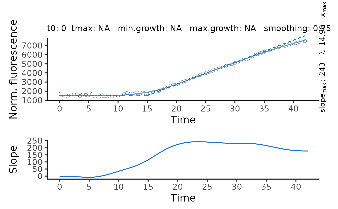
A flFitSpline object. The lag time is estimated as the intersection between the tangent at the maximum slope and the horizontal line with \(y = y_0\), where y0 is the first value of the dependent variable. Use plot.flFitSpline to visualize the spline fit and derivative over time.

x.in: Raw x values provided to the function as time or growth.
fl.in: Raw fluorescence data provided to the function as fl_data.
raw.x: Filtered x values used for the spline fit.
raw.fl: Filtered fluorescence values used for the spline fit.
ID: (Character) Identifies the tested sample.
fit.x: Fitted x values.
fit.fl: Fitted fluorescence values.
parameters: List of determined parameters.

A: Maximum fluorescence.
dY: Difference in maximum fluorescence and minimum fluorescence.
max_slope: Maximum slope of fluorescence-vs.-x data (i.e., maximum in first derivative of the spline).
x.max: Time at the maximum slope.
lambda: Lag time.
b.tangent: Intersection of the tangent at the maximum slope with the abscissa.
max_slope2: For biphasic course of fluorescence: Maximum slope of fluorescence-vs.-x data of the second phase.
lambda2: For biphasic course of fluorescence: Lag time determined for the second phase.
x.max2: For biphasic course of fluorescence: Time at the maximum slope of the second phase.
b.tangent2: For biphasic course of fluorescence: Intersection of the tangent at the maximum slope of the second phase with the abscissa.
integral: Area under the curve of the spline fit.

spline: smooth.spline object generated by the smooth.spline function.
spline.deriv1: list of time ('x') and growth ('y') values describing the first derivative of the spline fit.
reliable: (Logical) Indicates whether the performed fit is reliable (to be set manually).
fitFlag: (Logical) Indicates whether a spline fit was successfully performed on the data.
fitFlag2: (Logical) Indicates whether a second phase was identified.
control: Object of class fl.control containing list of options passed to the function as control.

Details

If biphasic = TRUE, the following steps are performed to define a second phase:

Determine local minima within the first derivative of the smooth spline fit.
Remove the 'peak' containing the highest value of the first derivative (i.e., \(mu_{max}\)) that is flanked by two local minima.
Repeat the smooth spline fit and identification of maximum slope for later time values than the local minimum after \(mu_{max}\).
Repeat the smooth spline fit and identification of maximum slope for earlier time values than the local minimum before \(mu_{max}\).
Choose the greater of the two independently determined slopes as \(mu_{max}2\).

Examples

# load example dataset
input <- read_data(data.growth = system.file('lac_promoters.xlsx', package = 'QurvE'),
                   data.fl = system.file('lac_promoters.xlsx', package = 'QurvE'),
                   sheet.growth = 1,
                   sheet.fl = 2 )
#> Sample data are stored in columns. If they are stored in row format, please run read_data() with data.format = 'row'.

# Extract time and normalized fluorescence data for single sample
time <- input$time[4,]
data <- input$norm.fluorescence[4,-(1:3)] # Remove identifier columns

# Perform linear fit
TestFit <- flFitSpline(time = time,
                       fl_data = data,
                       ID = 'TestFit',
                       control = fl.control(fit.opt = 's', x_type = 'time'))

plot(TestFit)