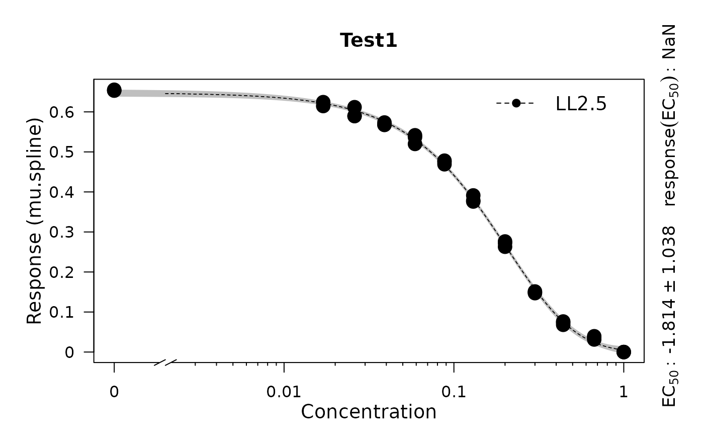
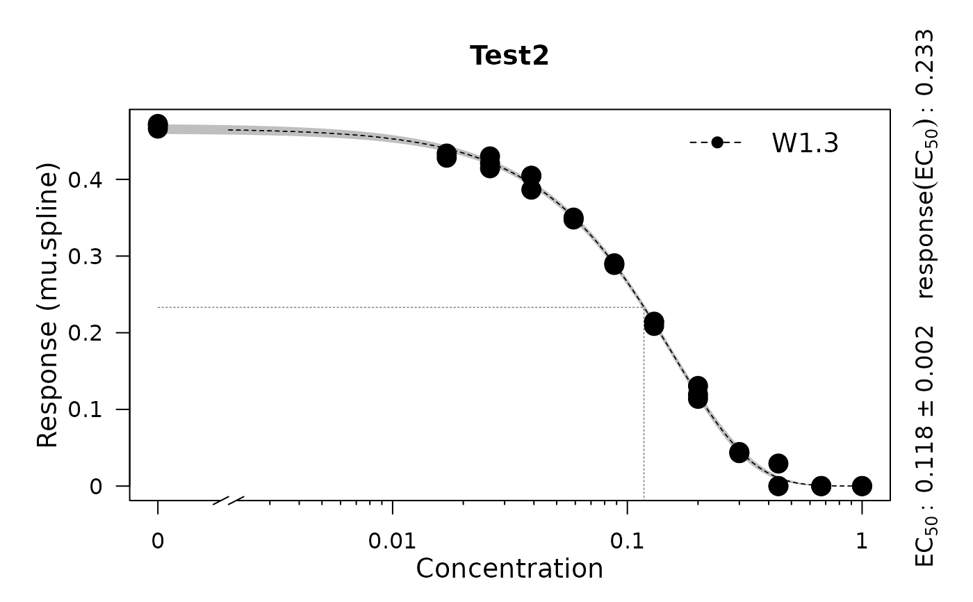
Generic plot function for drFit objects.

codeplot.drFit calls codeplot.drFitSpline for each group used in a dose-response analysis

Usage

# S3 method for drFit
plot(
  x,
  combine = TRUE,
  names = NULL,
  exclude.nm = NULL,
  pch = 16,
  cex.point = 2,
  basesize = 15,
  colors = NULL,
  lwd = 0.7,
  ec50line = TRUE,
  y.lim = NULL,
  x.lim = NULL,
  y.title = NULL,
  x.title = NULL,
  log.y = FALSE,
  log.x = FALSE,
  plot = TRUE,
  export = FALSE,
  height = NULL,
  width = NULL,
  out.dir = NULL,
  out.nm = NULL,
  ...
)

Arguments

x: object of class drFit, created with growth.drFit.
combine: (Logical) Combine the dose-response analysis results of all conditions into a single plot (TRUE) or not (FALSE).
names: (String or vector of strings) Define conditions to combine into a single plot (if combine = TRUE). Partial matches with sample/group names are accepted. If NULL, all samples are considered. Note: Ensure to use unique substrings to extract groups of interest. If the name of one condition is included in its entirety within the name of other conditions, it cannot be extracted individually.
exclude.nm: (String or vector of strings) Define conditions to exclude from the plot (if combine = TRUE). Partial matches with sample/group names are accepted.
pch: (Numeric) Shape of the raw data symbols.
cex.point: (Numeric) Size of the raw data points.
basesize: (Numeric) Base font size.
colors: (Numeric or character) Define colors for different conditions.
lwd: (Numeric) Line width of the individual splines.
ec50line: (Logical) Show pointed horizontal and vertical lines at the EC50 values (TRUE) or not (FALSE).
y.lim: (Numeric vector with two elements) Optional: Provide the lower (l) and upper (u) bounds on the y-axis as a vector in the form c(l, u). If only the lower or upper bound should be fixed, provide c(l, NA) or c(NA, u), respectively.
x.lim: (Numeric vector with two elements) Optional: Provide the lower (l) and upper (u) bounds on the x-axis as a vector in the form c(l, u). If only the lower or upper bound should be fixed, provide c(l, NA) or c(NA, u), respectively.
y.title: (Character) Optional: Provide a title for the y-axis.
x.title: (Character) Optional: Provide a title for the x-axis.
log.y: (Logical) Log-transform the y-axis of the plot (TRUE) or not (FALSE)?
log.x: (Logical) Log-transform the x-axis of the plot (TRUE) or not (FALSE)?
plot: (Logical) Show the generated plot in the Plots pane (TRUE) or not (FALSE).
export: (Logical) Export the generated plot as PDF and PNG files (TRUE) or not (FALSE).
height: (Numeric) Height of the exported image in inches.
width: (Numeric) Width of the exported image in inches.
out.dir: (Character) Name or path to a folder in which the exported files are stored. If NULL, a "Plots" folder is created in the current working directory to store the files in.
out.nm: (Character) The name of the PDF and PNG files if export = TRUE. If NULL, a name will be automatically generated including the chosen parameter.
...: Additional arguments. This has currently no effect and is only meant to fulfill the requirements of a generic function.

Value

One plot per condition tested in the dose-response analysis or a single plot showing all conditions if control = growth.control(dr.method = "spline") was used in growth.drFit and combine = TRUE.

Examples

# \donttest{
# Create random growth data set
rnd.data1 <- rdm.data(d = 35, mu = 0.8, A = 5, label = "Test1")
rnd.data2 <- rdm.data(d = 35, mu = 0.6, A = 4.5, label = "Test2")

rnd.data <- list()
rnd.data[["time"]] <- rbind(rnd.data1$time, rnd.data2$time)
rnd.data[["data"]] <- rbind(rnd.data1$data, rnd.data2$data)

# Run growth curve analysis workflow
gcFit <- growth.gcFit(time = rnd.data$time,
                       data = rnd.data$data,
                       parallelize = FALSE,
                       control = growth.control(fit.opt = "s",
                                                suppress.messages = TRUE))

# Perform dose-response analysis
drFit <- growth.drFit(gcTable = gcFit$gcTable,
                 control = growth.control(dr.parameter = "mu.spline"))
#> 
#> === EC 50 Estimation ==============================
#> ---------------------------------------------------
#> --> Checking data ...
#> --> Number of distinct tests found: 2 
#> --> Valid datasets per test: 
#>       TestID Number
#>       Test1  35    
#>       Test2  35    
#> Warning: NaNs produced

# Inspect results
summary(drFit)
#>    Test log.x log.y Samples EC50.Estimate EC50.Std..Error EC50.Lower EC50.Upper
#> 1 Test1 FALSE FALSE       0    -1.8136354     1.037698650 -3.9328988  0.3056280
#> 2 Test2 FALSE FALSE       0     0.1178171     0.001706518  0.1143411  0.1212932
#>       yEC50      test model
#> 1       NaN mu.spline LL2.5
#> 2 0.2331317 mu.spline  W1.3

plot(drFit)


# }