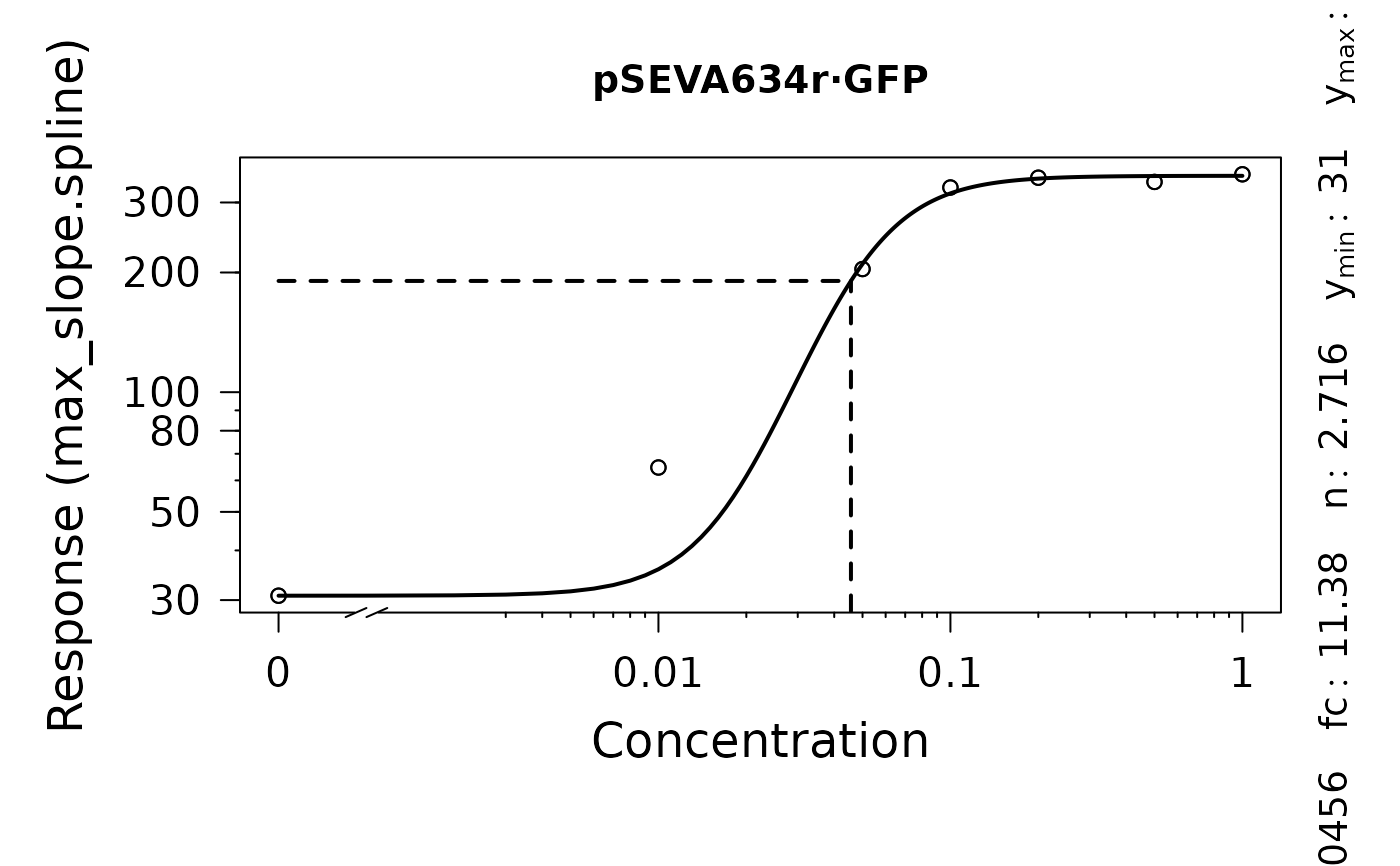
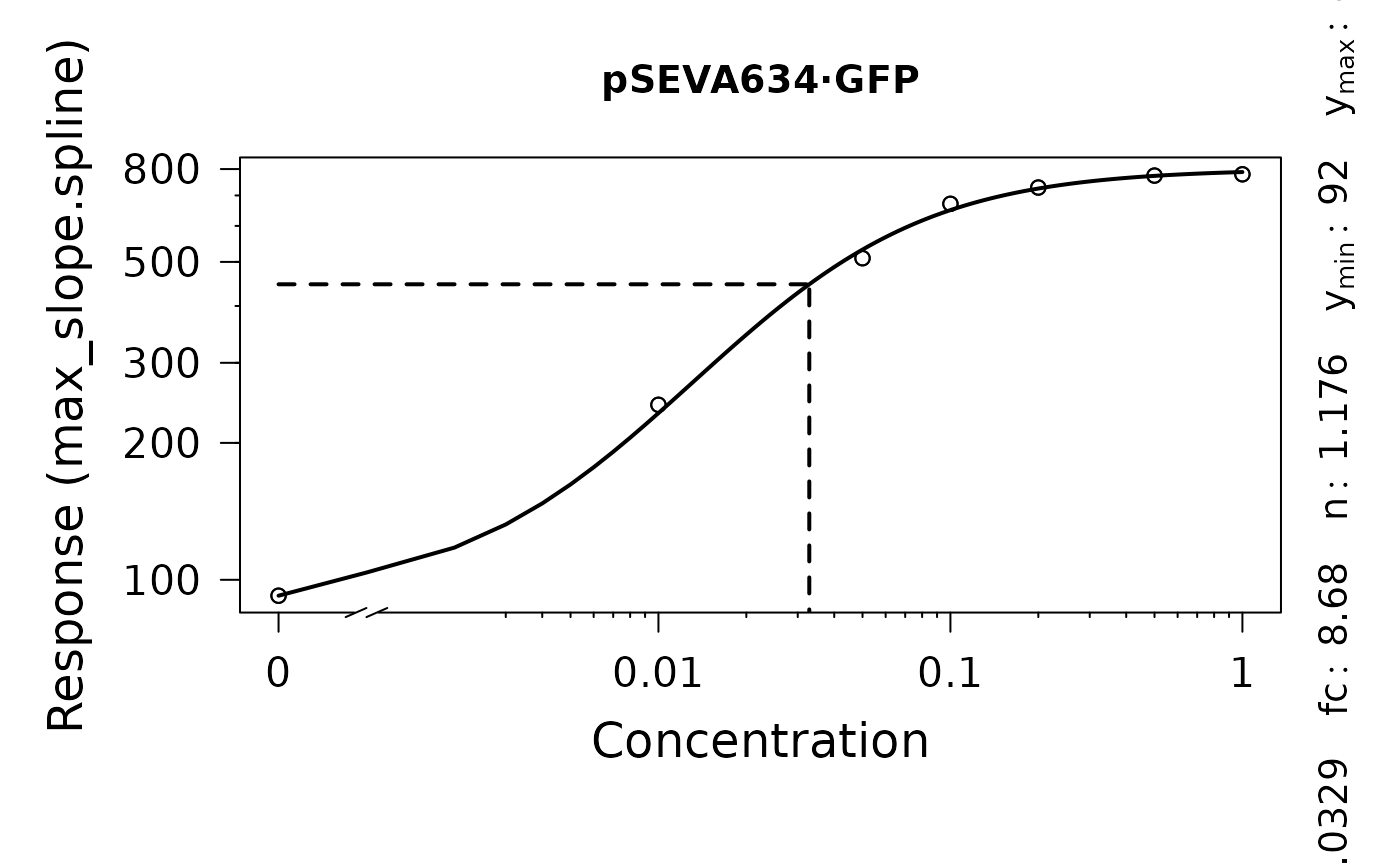
codedrFitfl calls plot.drFitFLModel for each group used in a dose-response analysis with dr.method = "model"
Arguments
- x
object of class
drFit, created withgrowth.drFit.- ec50line
(Logical) Show pointed horizontal and vertical lines at the EC50 values (
TRUE) or not (FALSE).- log
(Character) String which contains '"x"' if the x axis is to be logarithmic, '"y"' if the y axis is to be logarithmic and '"xy"' or '"yx"' if both axes are to be logarithmic. The default is "x". The empty string "" yields the original axes.
- pch
(Numeric) Shape of the raw data symbols.
- broken
(Logical) If TRUE the x axis is broken provided this axis is logarithmic (using functionality in the CRAN package 'plotrix').
- bp
(Numeric) Specifying the break point below which the dose is zero (the amount of stretching on the dose axis above zero in order to create the visual illusion of a logarithmic scale including 0). The default is the base-10 value corresponding to the rounded value of the minimum of the log10 values of all positive dose values. This argument is only working for logarithmic dose axes.
- n.xbreaks
(Numeric) Number of breaks on the x-axis (if not log-transformed). The breaks are generated using
pretty. Thus, the final number of breaks can deviate from the user input.- n.ybreaks
(Numeric) Number of breaks on the y-axis (if not log-transformed). The breaks are generated using
pretty. Thus, the final number of breaks can deviate from the user input.- colSpline
(Numeric or character) Spline line colour.
- colData
(Numeric or character) Contour color of the raw data circles.
- cex.point
(Numeric) Size of the raw data points.
- cex.lab
(Numeric) Font size of axis titles.
- cex.axis
(Numeric) Font size of axis annotations.
- y.lim
(Numeric vector with two elements) Optional: Provide the lower (
l) and upper (u) bounds on the y-axis as a vector in the formc(l, u). If only the lower or upper bound should be fixed, providec(l, NA)orc(NA, u), respectively.- x.lim
(Numeric vector with two elements) Optional: Provide the lower (
l) and upper (u) bounds on the x-axis as a vector in the formc(l, u). If only the lower or upper bound should be fixed, providec(l, NA)orc(NA, u), respectively.- lwd
(Numeric) Line width of the individual splines.
- plot
(Logical) Show the generated plot in the
Plotspane (TRUE) or not (FALSE).- export
(Logical) Export the generated plot as PDF and PNG files (
TRUE) or not (FALSE).- height
(Numeric) Height of the exported image in inches.
- width
(Numeric) Width of the exported image in inches.
- out.dir
(Character) Name or path to a folder in which the exported files are stored. If
NULL, a "Plots" folder is created in the current working directory to store the files in.- ...
Additional arguments. This has currently no effect and is only meant to fulfill the requirements of a generic function.
Value
One plot per condition tested in the dose-response analysis (fl.drFit with control = fl.control(dr.method = "model")).
Examples
# load example dataset
input <- read_data(data.growth = system.file("lac_promoters.xlsx", package = "QurvE"),
                   data.fl = system.file("lac_promoters.xlsx", package = "QurvE"),
                   sheet.growth = 1,
                   sheet.fl = 2 )
#> Sample data are stored in columns. If they are stored in row format, please run read_data() with data.format = 'row'.

# Define fit controls
control <- fl.control(fit.opt = "s",
             x_type = "time", norm_fl = TRUE,
             dr.parameter = "max_slope.spline",
             dr.method = "model",
             suppress.messages = TRUE)

# Run curve fitting workflow
res <- flFit(fl_data = input$norm.fluorescence,
             time = input$time,
             parallelize = FALSE,
             control = control)

# Perform dose-response analysis with biosensor model
drFitfl <- fl.drFit(flTable = res$flTable, control = control)

plot(drFitfl)


