Generic plot function for flcFittedLinear objects. Plot the results of a linear regression on ln-transformed data

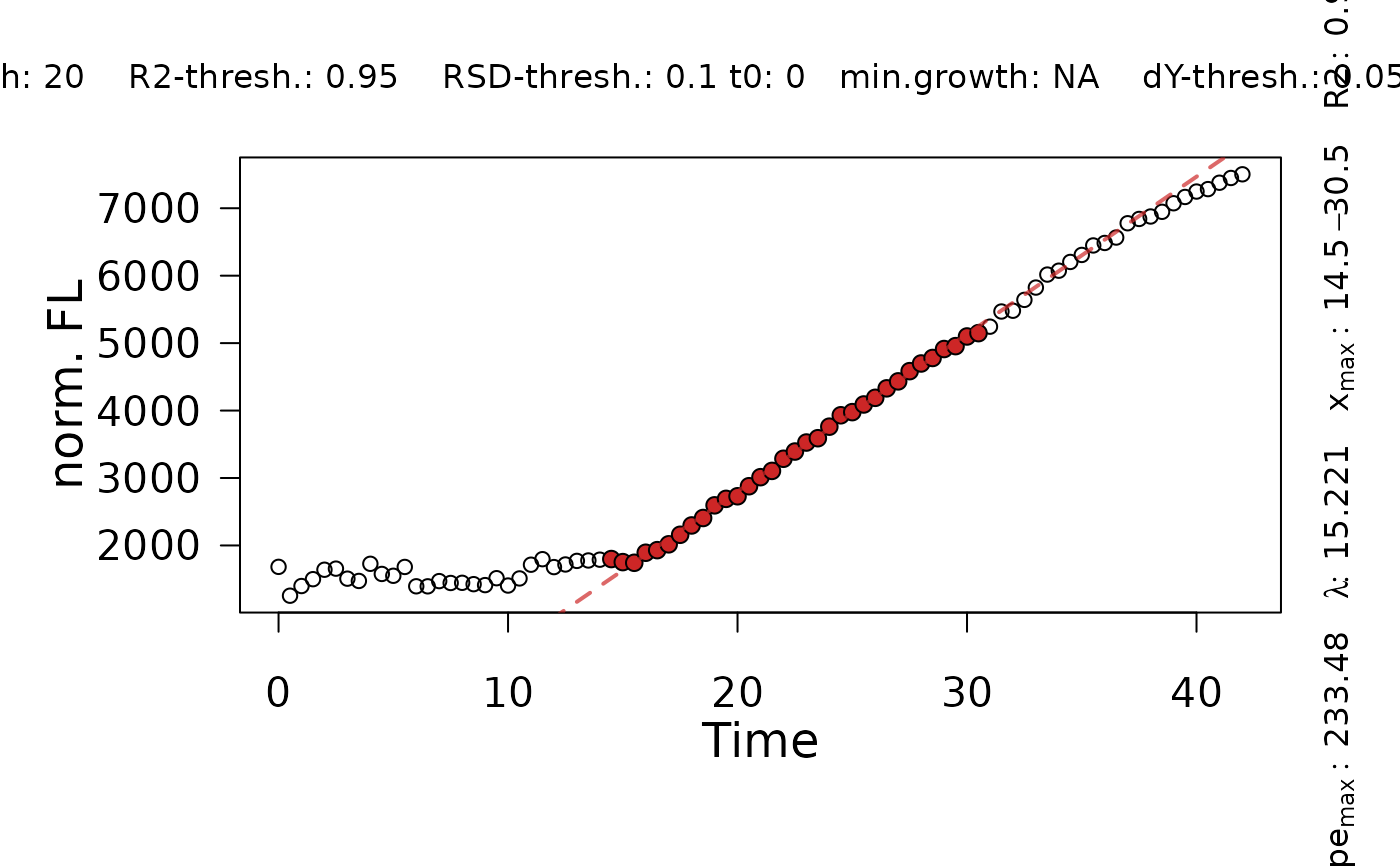
plot.flFitLinear shows the results of a linear regression and visualizes raw data, data points included in the fit, the tangent obtained by linear regression, and the lag time.

Usage

# S3 method for flFitLinear
plot(
  x,
  log = "",
  which = c("fit", "diagnostics", "fit_diagnostics"),
  pch = 21,
  cex.point = 1,
  cex.lab = 1.5,
  cex.axis = 1.3,
  lwd = 2,
  color = "firebrick3",
  y.lim = NULL,
  x.lim = NULL,
  plot = TRUE,
  export = FALSE,
  height = ifelse(which == "fit", 7, 5),
  width = ifelse(which == "fit", 9, 9),
  out.dir = NULL,
  ...
)

Arguments

x: A flFittedLinear object created with flFitLinear or stored within a flFitRes or flFit object created with fl.workflow or flFit, respectively.
log: ("x" or "y") Display the x- or y-axis on a logarithmic scale.
which: ("fit" or "diagnostics") Display either the results of the linear fit on the raw data or statistical evaluation of the linear regression.
pch: (Numeric) Shape of the raw data symbols.
cex.point: (Numeric) Size of the raw data points.
cex.lab: (Numeric) Font size of axis titles.
cex.axis: (Numeric) Font size of axis annotations.
lwd: (Numeric) Line width.
color: (Character string) Enter color either by name (e.g., red, blue, coral3) or via their hexadecimal code (e.g., #AE4371, #CCFF00FF, #0066FFFF). A full list of colors available by name can be found at http://www.stat.columbia.edu/~tzheng/files/Rcolor.pdf
y.lim: (Numeric vector with two elements) Optional: Provide the lower (l) and upper (u) bounds on y-axis as a vector in the form c(l, u).
x.lim: (Numeric vector with two elements) Optional: Provide the lower (l) and upper (u) bounds on the x-axis as a vector in the form c(l, u).
plot: (Logical) Show the generated plot in the Plots pane (TRUE) or not (FALSE).
export: (Logical) Export the generated plot as PDF and PNG files (TRUE) or not (FALSE).
height: (Numeric) Height of the exported image in inches.
width: (Numeric) Width of the exported image in inches.
out.dir: (Character) Name or path to a folder in which the exported files are stored. If NULL, a "Plots" folder is created in the current working directory to store the files in.
...: Further arguments to refine the generated base R plot.

Value

A plot with the linear fit.

Examples

# load example dataset
input <- read_data(data.growth = system.file("lac_promoters.xlsx", package = "QurvE"),
                   data.fl = system.file("lac_promoters.xlsx", package = "QurvE"),
                   sheet.growth = 1,
                   sheet.fl = 2 )
#> Sample data are stored in columns. If they are stored in row format, please run read_data() with data.format = 'row'.

# Extract time and normalized fluorescence data for single sample
time <- input$time[4,]
data <- input$norm.fluorescence[4,-(1:3)] # Remove identifier columns

# Perform linear fit
TestFit <- flFitLinear(time = time,
                       fl_data = data,
                       ID = "TestFit",
                       control = fl.control(fit.opt = "l", x_type = "time",
                       lin.R2 = 0.95, lin.RSD = 0.1,
                       lin.h = 20))

plot(TestFit)